What Equal Pay methodologies are out there?
In our previous blog post we explored the value of using an advanced equal pay methodology: it offers deeper insights into the root causes of pay gaps and supports with legislation like the EU Pay Transparency Directive. That naturally leads to the next question: what methodologies are available? In this blog post, we share with you several methods we have come across in our field of work.
Side note. In this blog series, we take the gender equal pay analysis as an example, but of course also other (two) groups can be compared, for example Western versus non-Western employees.

When it comes to equal pay methodologies, there are two directions that can be taken: regression-based or weighing-based.
Let’s first discuss the regression-based techniques:
- One of the most commonly used techniques to perform an equal pay analysis is Multiple Linear Regression (MLR). This method helps us understand how different factors influence salary by building a statistical model, a mathematical equation, that predicts salary based on various employee characteristics.
For example, the model might look at variables such as job level and years of experience. These variables are included because they are legitimate factors that typically influence pay.
The equation might look something like this:
salary = β₀ + β₁*(job level) + β₂*(years of experience) + ... + βn*(gender) + ε
From this you can see for example that for each added year of experience, the salary will be increased with β₂. So, if β₂ would equal 350, it would mean that for every added year of experience, the individual’s salary would increase with 350 euro.*
What stands out in this model is that gender is included as one of the variables. Not because it should influence pay, but because we want to measure if it does. The coefficient associated with gender (βn) tells us whether after accounting for all other factors, there is still a pay difference between men and women.
* Certain assumptions need to be met in the data to be able to apply regression techniques. For Equal pay this means we must use the natural log to log-transform the dependent variable: salary. Consequently, the coefficients in the model do not represent an amount in euros, but a percentage: if β₂ would equal 0.03, it would mean that with every added year of experience, the individual’s salary would increase with (approximately) (e^0.03=) ±3%.
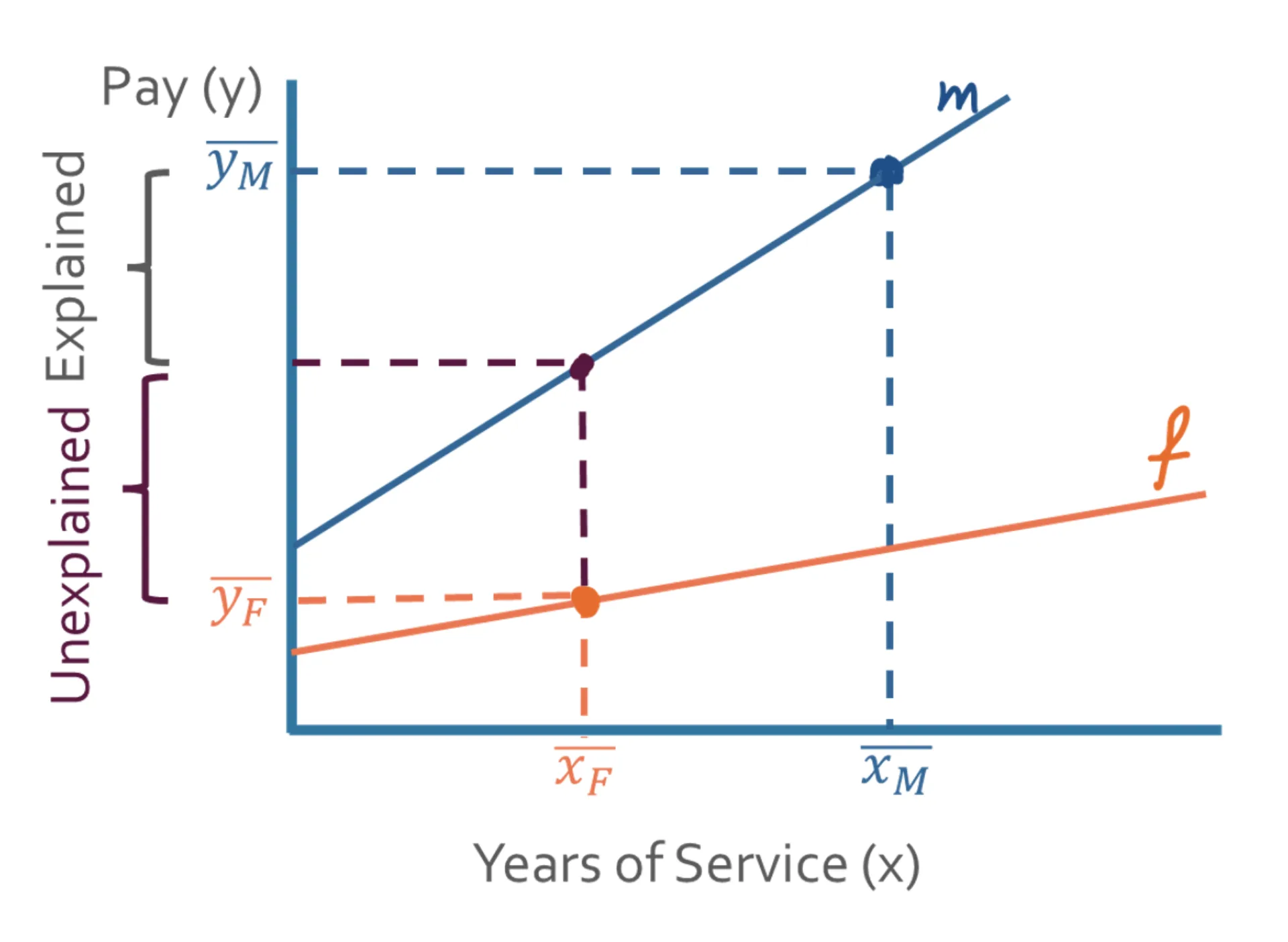
- Another approach is to build separate MLR models for men and women and then compare the predicted salaries for an "average" male and an "average" female based on their respective models. The difference between these two predicted salaries can be broken down into two parts: [1] an explained part and [2] an unexplained part. To obtain these parts, the average female is projected on the model of the males. See below a simplified illustration with one variable:

The ”m” and ”f” lines in the image above are respectively the male and female model. The values on the x-axis represent the years of service of the average female (F) and the average male (M), and the values on the y-axis represent their average pay.
The difference between the average female’s salary on the male model and average male’s salary thereon, is the explained part. Namely, this explained part reflects differences in characteristics, in this case years of experience, that justify a pay difference.
The unexplained part, on the other hand, cannot be attributed to measurable factors. In the example, there is no difference in years of service, yet the average female salary on the female model is lower than the salary on the male model. This is considered the corrected gender pay gap, or in other words, the equal pay gap.
This technique is known as the Oaxaca-Blinder Decomposition (OBD), and it is a widely used method in labor economics to analyze wage disparities between groups.
For the last regression method, we exclude gender from the model entirely. Instead, we predict a salary for each employee based solely on objective factors such as job level and years of experience. We then compare each employee’s actual salary to their predicted salary. By analyzing the average difference between predicted and actual salaries for men and women, we can identify an equal pay gap.
- We refer to this technique as the pay prediction approach.
Then the weighing-based technique:
Our Rake method. In this approach, each individual is assigned a weight to ensure that the distribution of background characteristics, such as job level and years of experience, is statistically equal between the male and female groups.

By applying these weights, we effectively create a scenario in which the two groups are comparable. We can then calculate the equal pay gap using the same simple formula for calculating the gender pay gap but now based on the average weighted salaries.
Now that we have explored the main methodologies, what is next?
In the upcoming posts of this series, we will explore the strengths and weaknesses of each approach to help you determine which method best aligns with your organization’s needs and objectives.
Related Insights
